Uncategorized

Data Description: Slave Sales 1775-1885

For my final project I decided to discuss the slave sales between 1775-1885. While working on this project, I noticed several correlations as well as other factors that I hadn’t thought of before. My data for this project is a combination of numeric, textual, as well as geographic data. The numeric perspective of the data stems from the appraised value that the slaves are given in the data set. Another way that numeric data is used in this data set are the years. There is a gradual increase in the years from 1775 all the way to 1885. In addition to the years throughout slavery there is a date of entry and age groups of the slaves are included in the data. On the textual aspect of the data set there is an abundance of information that is conveyed through the text. There are text data on the sheet such as gender of the slaves, any defects that these slaves may or may not have, and any skills that some of these slaves may or may not posses. An example of the text data portion of the sheet would be something like “Deaf” or ” house servant” that is included on the data sheet. And the last aspect of data conveyed on the data sheet is geographic portion. The way that the data sheet puts this information out is through the locations in the United States that the slaves are residing in and where they are working at. The geography portion of the data from the sheet is the smallest data set of the three. The geography only has two sets; State and county. Despite only geography having two sets, it is involved in most of the visual sheets within the project. The columns in the data set mostly consists of slave gender, state code, age, skills, and date entry. The gender is the sex of each slave that is accounted for within the data provided. A popular trend between sex and value is heavily noted in the data set. Perhaps the biggest relationship between sex and value that someone with little prior knowledge can infer would be that the male slaves would be appraised at a higher amount than their female counterparts. The state code is which state in which whom the slaves belong to while the county is which part of that state the slaves belong to. There are an array of states that are included in the data sheet. The states range from those states that are deep south to those that are more up north border lining slave state and free state. The age column consists of the different age ranges between the slaves. The skills portion of the columns are used to state if the slaves have a special skill which may add to their value. Lastly the date of entry are the dates that have been recorded in which the slaves are enslaved or born. The rows are mostly made up of the average appraisal value of the slaves. Sometimes the row would include one of the options that are in the columns as well.

2 data visualizations 

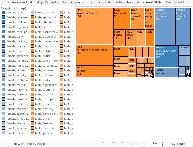
For my first visual, I have chosen to use the data that I created using the skills and values of the slaves depending on what state that they live in. The story told in this data visual is how much of an asset that these slaves were to the productivity of not only the states in the south, but to the United States as a whole and therefore made how much they were considered to be worth increased based on said skills. Each of these states in the south had different appraisal value of their slaves depending on what skills that the slaves had. Some of these skills were more challenging than others such as a slave with the “construction” skill will be at a higher appraisal value than a “cigar maker”. It’s only natural that the slaves who are more diverse in the jobs they can do and the level of difficulty of the job makes them worth a little more than their counterparts who aren’t as well rounded or who don’t have any skills that can be deemed as challenging. An observation that I made in the data set is that the states of Louisiana and Mississippi have the highest appraisal value of there slaves each skill category that they are in. When the states of Louisiana and Mississippi where in the same category, the state of Mississippi had a higher appraisal value than Louisiana. Perhaps the reason that the states of Mississippi and Louisiana have their slaves at a much higher value than the other states is because there was a heavy reliance in these slaves and their challenging skills that they possessed. These two states are known for their giant plantations and needed the man power to keep them up and running successfully. The slaves who can do the challenging task such as “construction”, “blacksmith” and “carpenter or cabinet maker” are viewed as a bigger asset to the slave owners and the well being of the plantation as a whole. Unlike Mississippi however, Louisiana has slaves of every skill set. With this observation, the state of Louisiana has the biggest diversity of slaves with skills. Louisiana finds it necessary to have slaves of every skill set because they may find it important to keep their economy up and running. The state of Maryland however is comprised of slaves that posses easier skills such as “Butler” and “house servant” . With slaves who posses these skills, Maryland has them set at a lower value since the skills aren’t as desirable. States such as Maryland that are located more towards the north perhaps didn’t need the same slaves that their southern counterparts needed as far as skills are concerned.  The northern states aren’t going to need slaves with the skill set of “field worker” since there aren’t any plantations in the slave states that are more up north like the ones located in the south. The slaves located more to the northern states appear to have skill sets that are more like “chores” as opposed to hard labor.

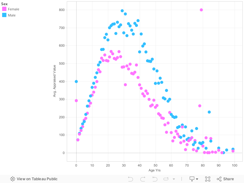
For the second visual that I decided to go with is the average sale appraisal of slaves. What I did with this visualization is separate the slaves by sex as well as what state that each sex resided in. As expected, the male slaves are valued at a much higher price than the female slaves on average. The male slaves were valued at almost a hundred dollars more than the female slaves were valued at by most of the states that were included in the data sheet. One thing that I found that was surprising while looking through the data was that female slaves are held at an higher appraisal value than male slaves in one state. while doing this project I didn’t expect to see female slaves being valued more than male slaves at all. The one state that female slaves are valued more is South Carolina. Not only are the female slaves valued more in this state than the males but they are also more by a significant amount. The female slaves in South Carolina are well over a hundred dollars more than the male slaves. This could be due to the fact that there isn’t as many labor inducing jobs in this state. Another factor for this higher appraisal could be a scarcity of female slaves in this state for some unknown reason.  As far as male appraisal goes, it should come as no surprise that the state of Mississippi has the higher appraisal of male slaves. It is a known fact that Mississippi is one of the two plantation giants of the south during this time frame along with the state of Louisiana. As depicted on the visualization on top, these two states are diverse in the skill sets of their slaves as well as having slaves that can perform difficult tasks which reflect the appraisal value of these slaves. But what I also found was that Mississippi also has the highest appraisal value of female slaves as well. Mississippi relied heavy on slaves so this can be he reason why they are valued so much.  Another finding in the data sheet that I observed was the low appraisal rate of both male and female slaves that the state of Maryland has. Again, as depicted in the visualization above the low appraisal rate of slaves in Maryland shouldn’t be surprising. The state of Maryland has a slave appraisal value under two hundred dollars. The story of Maryland seems pretty straight forward and simple. Maryland didn’t own any plantations or any fields that required slaves to be in and maintain; but what Maryland did have was wealthy white people who would purchase these slaves to perform the task and daily chores that they themselves didn’t want to do such as gardening or household chores. Maryland doesn’t need slaves that are as skillful as those that are located more towards the south which explains for the low appraisal. It seems to me that the state of Maryland has slaves just because it is legal to have them and do not rely heavily on them and they seemed more as a luxury.

 

 

 

Process documentation 

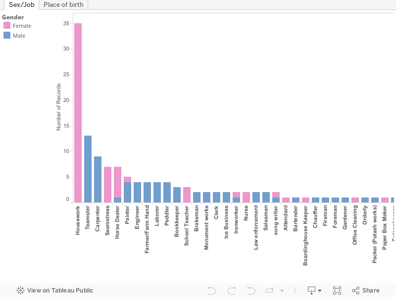
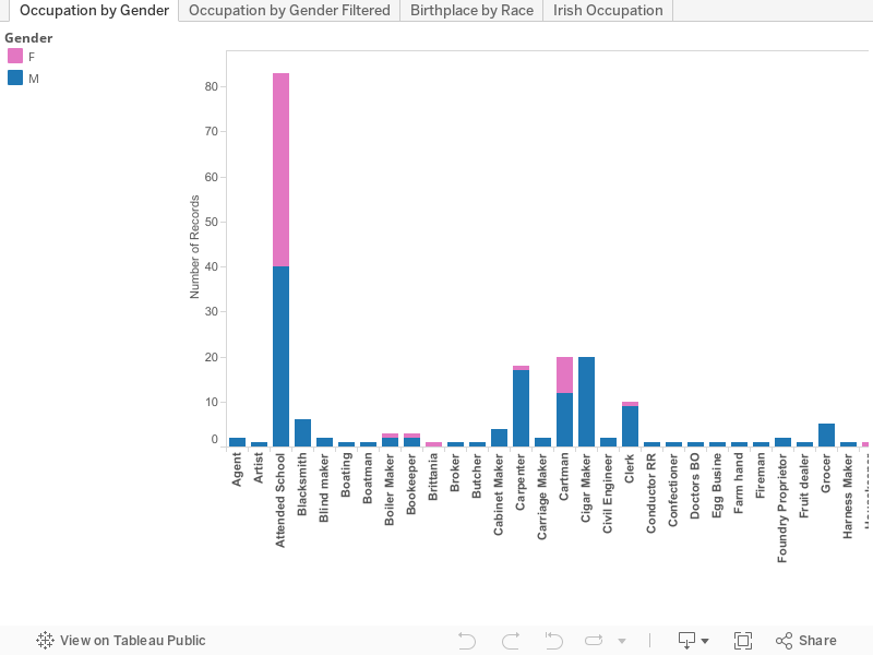
In order to make my visualizations I had to take a few different approaches. Some methods were more effective at conveying the information than others. I didn’t want to focus on one particular style of visualization because I felt that it would bore the reader and therefore the overall message that I’m trying to put out will get lost. I used several different kinds of graphs and charts in my final project but I’m going to focus on the two prominent methods that appear more frequent than the others. The two that I’m going to focus on are the bar graphs and line graphs. The first visualization type that I chose to use was the simple bar graph. I believe the bar graph is one of the best methods in showing data. It’s simple to read and easy to create. I use the bar graph to compare several factors such as differences in sexes between the slaves in the data set, the appraisal value of the slaves as well as what state or counties these slaves reside in, and that’s only in the first appearance of the bar graph.

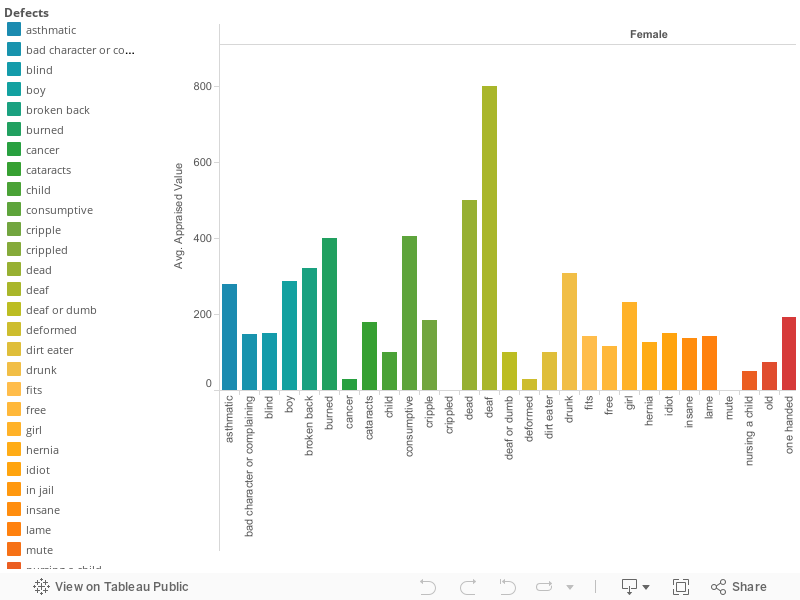
Another variation of the bar graph that I used was the stacked bar graph. Slightly odd at first but turned out to be very effective. With this graph I was able to compare the skills of each slaves and determine an average value of them by location. The stacked bar graph option made it easier to display this information than another visual type may have been. In regards to what color of the bar graphs I chose and decide to use depends on the information from the data sheet that I plan on highlighting. For the ” Slave appraisal” data chart I decided to go with black with the intentions to have the reader notice the color of these enslaved men and women looking at the prices that they were being auctioned off. For the “skills & values by state” it may be hard to read at first glance because there are so many colors but it gets easy to understand after a minute. I used multiple colors because there is more information that has to be displayed. The skills are color coated by state to and the skills are located on the X-axis. The bar graph may be the best method for comparing data that I have ever used. The stacked bar graph helps argue that slaves are appraised differently based on sex as well as skill and location.

 

Argumentation

The causation of the appraisal for female and male slaves in the slave data is the high demand for slaves between 1775 and 1885 due to the economic opportunity that the southern states had at the time in which were created through the means of producing goods such as cotton and tobacco. Slaves have fluctuated in value over that hundred year span, mostly increasing in value as the years went on. It has become an ordinary way of living for those in the south to own slaves and benefit from their free labor. As the popularity of owning slaves grew, so did their value. In the beginning of the years in which the data was recorded, having slaves was legal and a way of life for the white men which mainly were located in the south. It is a pretty known fact that tobacco plants as well as other jobs were located in the southern states and that they took a lot of labor to maintain. With the legality of slaves, those who were able to afford slaves bought as many as they could to do these jobs that required an abundance of labor. The appraisal value of male slaves are more than that of female slaves. This is caused due to the amount of labor as well as type of labor that male slaves can do that female slaves can’t physically do. Females don’t have the same body type or muscle mass that males do, therefore they are more limited to the work they can do. Male slaves also tend to be more skillful with their hands and can do jobs such as being a blacksmiths while women who are skillful will most likely do the jobs such as basket making and other simple jobs. While males are doing more physical labor out in the field or blacksmith work, female slaves can do less physical work such as watching children, making items such as baskets, and other activities. With that being said, their value isn’t going to be as high because that labor isn’t as intense or challenging and isn’t as profitable as the males line of work is overall. It is pretty standard that all male slaves will be worth more money than their female counterparts. The direct causation of the value difference between the male and female values seems to be due solely to their potential productivity and how much money they can bring in.

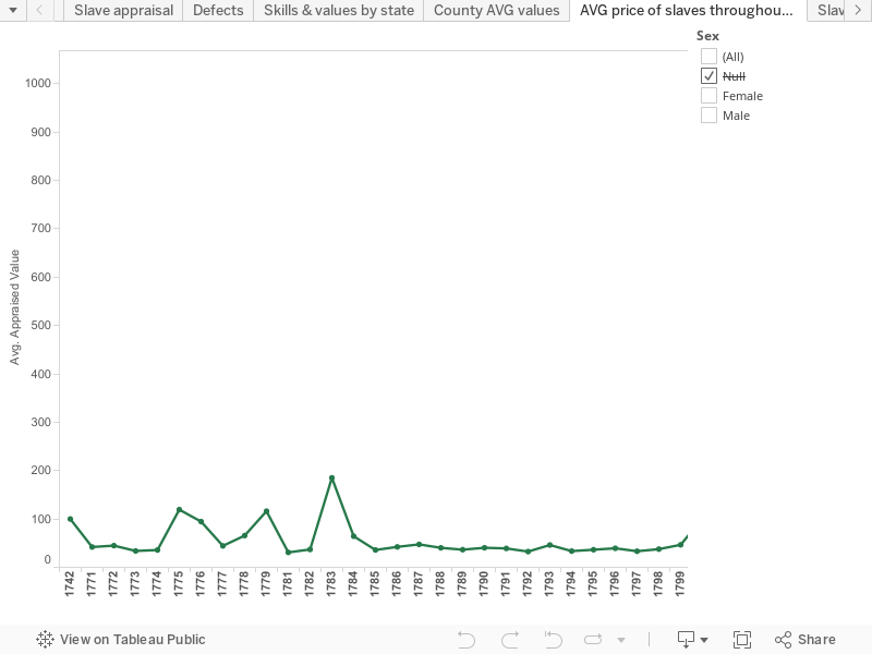
An argument that can be noted from the data set that may come as a surprise to some people is the average price of slaves throughout time. Most people will automatically assume that as the years go by that the value in slaves only increases until it is abolished in the 1860’s. According to the data however, the value trend with slaves throughout time haven’t been as consistent as some people may think. The trend of slave values started at a decent number and then proceeded to decrease in value before picking back up. It isn’t clear why the value of slaves decreased during this time but it can be argued that the causation for the slaves to steadily increase in value after it’s descent can be caused by the growing popularity of slaves. As the years went by, news of how effective the slaves were could have been spread throughout the south. The businesses started to thrive and become more successful than they may have been previously. It is noted that the value of slaves really started to get high in price in the 1800’s. The causation of this spike can be credited to the industrial revolution. The south was a big manufacturer of goods during this time period and provided these goods to the northern states; states in which slaves were outlawed. With the slaves providing free labor, the south was able to benefit exponentially. This of course made the south even more wealthy and this in turn caused the appraisal of slaves to increase since they were viewed as a great asset to the owner of the plantations and manufacturers of goods. Even though the value of slaves were at a higher average than it was previously, the value of slaves still drop in price certain years before increasing again. This trend of erratic values continues throughout the decades. The causation for this trend is unknown and there aren’t any signs that may explain why. The value of slaves however hits its peak in 1864 in which is a time in American history when the civil war was taking place. The average appraisal price for the slaves during this time period was over a staggering 1000 dollars. The price of slaves during the time of the civil war jumped up by over three hundred dollars.  The reason for this insanely high price can be argued to be a direct result of the civil war that was happening at this time. Since one of the main reasons of the civil war was over the liberation of slaves, this caused the value of the slaves to soar to new heights. This is the highest value that slaves have been since the data has been recorded. It can be inferred that slave owners were attempting to get top dollar for their slaves at this time since the possibility of slaves being outlawed all together was in the minds of the owners during the time of war if the south suffered defeat to the north. Slave owners figured that it was the best time to increase the value of their slaves in order to have some type of monetary gain in case the south lost the war. In the year 1885, the value of slaves appears to begin its plummet at a fast rate. This is a direct causation of the south losing the civil war to the north which resulted in the outlawing of slaves. Since having slaves were illegal, there was no longer an appraisal value on the now former slaves.

Further research questions 

The research conducted within the project brought about some research questions that may have not been thought about before hand.  One research question that was a result of the first visualization “Slave appraisal” would be since male slaves are worth more than female slaves, are they treated less harshly than female slaves; or is there no difference between the treatment of the slaves.  Perhaps the best way to go about answering this research question would be an attempt to find pictures as well as any documented treatment of both male and female slaves during the time of the census.

For the second visual “Skills & values by state” I learned a few new things and thought of some questions that this visualization forced me to think about. Before this project I had no idea that slaves had any skills. Before this data set I was under the misconception that all slaves did was pick cotton and serve as butlers ( for the lighter shade slaves). But according to the data there are an array of skills that these slaves possessed. But what exactly did these slaves do with their skills? For example, what did a slave with the skill of “construction” build? Do the slaves with the same skills work with each other or do they work on separate projects individually?  Trying to get answers for this research question may be a little challenging. It is unsure if any documents of what the slaves build will be recorded since slaves are generally viewed as “dumb”. During this time frame I find it unlikely that slaves would be credited with anything they have done.

My last visualization “AVG of slaves throughout the years” may be the most intriguing and thought provoking visual that I have used from the data set out of all the charts and graphs that I made. The reason I believe this to be the most interesting visual is due to the inconsistency of the data on the graph. This phenomena prompts several research questions due to the vast inconsistencies. One research question for this graph would be “Why doesn’t the price of slaves only increase since slaves were so widely used during this time period?” It seems a little strange that the price in slaves has periods in which it decreases in price before making it’s way back up. Several other research questions are “What causes these prices to drop?” “What was the cause for the prices of these slaves to increase again?” Just to focus on one year specifically for example purposes, the year “1783” increased dramatically from the previous year by well over a hundred dollars. But then the very next year the average value of slaves drops severely all the way to about sixty dollars. To go about answering these research I would have to visit a library or database hat has records of what may have occurred during this time span. Then focus more specifically on the year in which the data makes a dramatic change and see if there is any correlation within Americas history and the decrease or increase in the value of slaves within that year.

Data Description

The data that is provided mostly consists of numeric and textual data however when the data is all put together, it paints a very detailed image. It contains very general categories that don’t get into the best detail of the individuals.
The first two columns include the soldier’s full first and last name. From just looking at the first two columns, you can gather a few pieces of information. One being that everyone in this militia were men. This doesn’t come as a surprise to me because of the time period. A second piece of information that sticks out comes from their last names. You can tell some of the individual’s backgrounds just by reading their last names. The next three columns are their enlistment dates. This is an interesting piece of interesting because we can now find out when a majority of these men decided to sign up for militia. We can use this data to see if something happened around the date of their enlistment that motivated them to sign up. We can also tell get an assumption of who is in charge of who by the seniority of the enlistment date. Generally speaking that is how the military works, there is a strong emphasis on seniority. The next column includes when the men were born. The maximum age given in this document is 58 years old while the youngest being only 16. The average age of this militia is 28.87766 which would be rounded up to 29. The next column tells us where they were born. I feel that this is one of the more interesting and important columns in this data set. We now know where these men come from and there’s a surprising amount of individuals who come from European countries who signed up for fight for their new home. Another surprising piece of information is that there’s quite a few men from Britain who have signed up to fight their home country. The following column is equally as interesting and that is their current jobs. For the most part, the men who have signed up come from bluer collar type jobs. There aren’t any many men signed up for the militia that have a prestigious type job where they would be making a lot of money for the time. This doesn’t come as a surprise though because they would most likely be against a change in government because that would most likely result in them having to change their business. The following two columns tells us who their officer in charge and which company they were part in. Unfortunately I didn’t find much use for this information mostly because for many of the enlistees, there were no information provided for their company and also I couldn’t find much information about the officers that were in charge of them. The remaining columns give details about their physical appearance. The following columns are very informative because it really helps paint a picture of what these men looked like for us. For example, the smallest height on this chart was recorded as 4 foot 11 while the tallest is 6 1/4 feet. The remaining three columns deal with their complexion, skin color, and eye color. For the complexion column, the men were generalized into a few general categories being dark, brown, fair, and a few others.
By reading this piece of data, one could get a very good feel about the current condition of the Militia during that time. Giving the sense that maybe they weren’t the largest, most intimidating group of guys. However they were brave enough to sign up to fight and defend the people that they care about.

Visualization 1

There are several stories that can be told from the Albany Militia Muster Roster. From how the small militia looked, to the jobs that they had in their normal lives. It’s very interesting to see where the individuals come from and how old they were when they originally enlisted.
There is certainly a lot of personal information provided in the roster that paints a very descriptive story. The story that one of my visual focuses on are the racial backgrounds. The story behind this visualization is to illustrate what the militia looked like during this time with focus on the skin color of these men. With a majority of this militia being black, I was curious as to why that was. Were these men forced into signing up or were they truly volunteering to fight for freedom that they weren’t even promised? And also what were the negative impacts of having men who were forced into signing up. This visualization provides us with a few possibilities as to how they go their numbers and how effective they were. If the men categorized as “Black, Brown, Negro, Dark and Swarthy” voluntarily signed up for this militia, then I would say that they were a pretty effective militia. My reasoning behind this is because if all these men chose to sign themselves up, they must feel that they have something to fight for and protect. Sadly, I don’t feel that this was a reason why a majority of these men signed up. On the other hand, if these men were forced to sign up because they were slaves and they were told to, then I would say that it would lessen their effectiveness. This is because they are a majority of the militia and since they are being forced to fight for something they may not believe in, then these men may not be entirely motivated to die for the cause. On the other hand, there is a possibility that these men were promised their freedom in exchange for enlisting. I feel that this is the sad reality of what happened, however I’m not sure if this would mean that they will readily put their life on the line for something that they were just “promised”.

<script type=’text/javascript’ src=’https://public.tableau.com/javascripts/api/viz_v1.js’></script><div class=’tableauPlaceholder’ style=’width: 982px; height: 742px;’><noscript><a href=”><img alt=’Sheet 1 ‘ src=’https:&#47;&#47;public.tableau.com&#47;static&#47;images&#47;Bo&#47;Book1_9909&#47;Sheet1&#47;1_rss.png’ style=’border: none’ /></a></noscript><object class=’tableauViz’ width=’982′ height=’742′ style=’display:none;’><param name=’host_url’ value=’https%3A%2F%2Fpublic.tableau.com%2F’ /> <param name=’site_root’ value=” /><param name=’name’ value=’Book1_9909&#47;Sheet1′ /><param name=’tabs’ value=’no’ /><param name=’toolbar’ value=’yes’ /><param name=’static_image’ value=’https:&#47;&#47;public.tableau.com&#47;static&#47;images&#47;Bo&#47;Book1_9909&#47;Sheet1&#47;1.png’ /> <param name=’animate_transition’ value=’yes’ /><param name=’display_static_image’ value=’yes’ /><param name=’display_spinner’ value=’yes’ /><param name=’display_overlay’ value=’yes’ /><param name=’display_count’ value=’yes’ /><param name=’showTabs’ value=’y’ /></object></div>

Process Documentation

I sorted and grouped the different complexions provided and assumed the description of the complexion correlated with their race. For example I grouped “Black, Brown, Negro, Dark and Swarthy” assuming that they are all African Americans. I also grouped “Fair, Pale, Ready, Reddy, Ruddy, and Sandy” with the assumption that they all are Caucasian. And then I left Indians alone because they are Native to the land. I also excluded “Freckled” and “Pockpitted” because they both can be used to describe Indians, Blacks and Whites. I thought that this would be an interesting way to sort this data because all of these individuals either made the voluntary decision to sign up for this Militia, were forced, or given some type of deal to join and they come from all walks of life. Especially during this time period, there was a very large gap in social equality between blacks, whites and Indians. One would assume that a majority of the soldiers on this muster roster would be White because they have a whole lot more to lose and they were treated a whole lot better by society. I would have thought that since society has been so oppressive towards African Americans, there would be a tremendous dividend between the two with the Whites in the majority. Much to my surprise, the African Americans were in the majority leading by well over 100. I found this very interesting and once I saw this, I had to ask myself was this all voluntary? Maybe it was and they just had a love for the country and a desire to defend it. Another interesting fact is that there was only individuals that fell under the category of “Indian”. However I will admit that I was not entirely surprised. Foreign powers were coming into their land and trying to control it. Why would they want to sign up for a fight that really has nothing to do with them because either way, there will be a foreign country controlling their way of life.
I decided to use a simple bar graph to illustrate the different groups because it’s a simple yet powerful image where you can tell which group of people made up the majority of the militia. I also chose to compare the groups by just the numbers so that people can easily see the numerical difference between the groups. I feel that there is a different impact on the viewer of the graph when they see the actual amount of people compared to it being a percentage.

Argumentation

During this time period, there were tensions growing between the colonies and their imperialistic government governing them from across the Atlantic Ocean. With things starting to heat up, it became clear that there was soon to be some bloodshed. With this in mind, both sides started to enlist troops to strengthen their forces. This was the main reason why there was a formation of the Albany militia because they knew very well that the fighting would soon come to them. A major event that made the Americans realize that they should prepare for something was the French and Indian War. Although the Americans fought along side the British against the French and Native Americans, things were still not right between the two and this feeling grew larger after the war. For one, the war had been incredibly costly. It had a sever impact on the British economy and the Brits believed that the Americans should help pay for it. [1] This idea would result in ridicules taxes like the Stamp Act, and the Sugar act. The stamp act was enacted in 1765 and required that almost everything printed be printed on stamped paper, which would be a direct tax on the people. This is one was in which the British Parliament felt that they could get the colonist to help pay for the war. [2] It was acts like this that finally put the colonists over the edge. It was also taxes like these that gave birth to the infamous “No taxation without representation”. However there’s one big question that is still not answered, why the African Americans made of a majority of the Militia? Both the British and the Colonists took advantage of enslaved men by promising their freedom in exchange for fighting for their armies. This explains why there were a large number of enlistees of Blacks in the Albany roster. During the course of the revolutionary war, an estimated total of 25,000 to 30,000 both free and enslaved black men fought in numerous battles for both sides. [3] Although many of these men have been oppressed and were slaves, they played a vital role in the gain of our independence and had very pivotal roles on the military that resulted in our freedom. “Blacks on either side served as infantrymen, spies, couriers, cooks and guides. Some were rewarded with their freedom.” [3] For example there was a slave named James who served the revolutionists as a spy during a very climatic time in the revolution. He pretended to enlist in the Loyalist army and then he relayed important military information to the Americans, which gave the Americans the advantage in battle.
Although many of these men didn’t truly volunteer to join the ranks, they still fought with true effort in order for the revolution to succeed. They were given a deal to for their freedom and many took that opportunity which explains why the number of black enlisted men outnumbers the whites.

Visualization 2

Where a person is born defines a lot about them, especially a soldier. If a Soldier feels that his homeland is under threat, he will be willing to sacrifice himself in order to defend it. That is usually what separates Soldiers from people who get paid to fight. There is a sense of pride, country and a need to defend it. A second part of the data set provided that I will be focusing on will where these soldiers come from. Whether they come from a foreign country, or they list that they come from one of the states, it tells a whole lot about them and their story. Where these soldiers come from and where they say they come from are very different and tells us a lot about themselves and their sense of nationalism. For example, if an individual says that they are from New York when they sign up, that person could be from another country however he has a strong sense of pride about his new-found home there for he is willing to fight for it. On the other hand, an individual who declares that he is from another country may not feel the same sense of pride. But it should go without being said that either way, any individual who signed up for the militia is brave.

<script type=’text/javascript’ src=’https://public.tableau.com/javascripts/api/viz_v1.js’></script><div class=’tableauPlaceholder’ style=’width: 982px; height: 742px;’><noscript><a href=”><img alt=’Sheet 2 ‘ src=’https:&#47;&#47;public.tableau.com&#47;static&#47;images&#47;Bo&#47;Book1_9909&#47;Sheet2&#47;1_rss.png’ style=’border: none’ /></a></noscript><object class=’tableauViz’ width=’982′ height=’742′ style=’display:none;’><param name=’host_url’ value=’https%3A%2F%2Fpublic.tableau.com%2F’ /> <param name=’site_root’ value=” /><param name=’name’ value=’Book1_9909&#47;Sheet2′ /><param name=’tabs’ value=’no’ /><param name=’toolbar’ value=’yes’ /><param name=’static_image’ value=’https:&#47;&#47;public.tableau.com&#47;static&#47;images&#47;Bo&#47;Book1_9909&#47;Sheet2&#47;1.png’ /> <param name=’animate_transition’ value=’yes’ /><param name=’display_static_image’ value=’yes’ /><param name=’display_spinner’ value=’yes’ /><param name=’display_overlay’ value=’yes’ /><param name=’display_count’ value=’yes’ /><param name=’showTabs’ value=’y’ /></object></div>

As you can see in the image, a majority of individuals from this roster identified themselves as either coming from Ireland or Germany followed by England. This doesn’t come as a surprise because a majority of the people who came to New York in the first place were from Europe. All of the following militiamen come from New York and the surrounding areas. The huge difference between New York born troops and European born militiamen has mostly to do with the age of the newly formed government and country. The younger population mostly make up the American born militiamen and on the other hand, the older are the majority and they are the first generation to colonies the new land. I would predict that in the following years as the war progressed, more and more New York born men would enlist because they would eventually be old enough to fight. Some people may ask why sign up to fight for a country and land where they aren’t even from? Surprisingly, 71 individuals were actually born in England and would be fighting their own homeland. Initially I would have thought that it would have been 2nd generation men signing up for the Militia to fight the British. I was pleasantly surprised when I saw that a majority of the soldiers were born in Europe. They all signed up to accomplish a common goal and were tired of being oppressed by an imperialist government governing them from across the Atlantic Ocean. I think that it’s very impressive that these people from all different backgrounds were able to come together in order to defend what they called their new homes.

Process Documentation

I created this visualization by grouping the men by areas where they say they come from. For example the men who were born in New York, I combined them into one group even though they may have said that they come from different countries. I did it this way because it shows a powerful image of where these men come from. And it’s important to see where a majority of these come from. It also shows how all of these men come from all different walks of life and it also paints an image in our mind of what the militia looked like. The larger and darker the boxes get means that more men come from what area. And it’s important to note that the larger, darker boxes are almost all European countries.

Argumentation

The Albany militia mustered men from all walks of life. The information provided paints a picture of a misfit group of men. They came from all different countries and came together to fight a common enemy. The formation of this militia was very important. Because this was a government ruled by the British parliament, they were unable to form their own military. Therefor they had to form this militia in order to protect themselves. Many of the men, especially the younger ones had little to no military training. On the other hand, there were few who were veterans from the Indian wars. [4]
Contrary to what I said earlier asking why men would sign up to fight against their own home land of England and whether or not it would hinder their commitment to the fight for freedom, the men who signed up for the militia were the most patriotic. As stated previously, there was no army for these men to enlist in to fight in yet however when this changed, many of these militiamen enlisted in the Continental Army. And since these militiamen were fighting since the beginning, they were filled with patriotism and truly had a desire for freedom. [4]
There are several events that led to these men from all different backgrounds to come together for a mutual cause. In general, all of the events were moves made by the British government that frustrated the 13 colonies and eventually resulted in them being fed up and enlisting in the ranks of the militia. One of the first things that the British government did was the proclamation of 1763. In this particular situation, King George lll essentially told the settlers that they cant settle west of the Appalachian Mountains without guaranteed protection (which they promised). This made the settlers unhappy with the government because it was their first attempt at interfering with the colonies. [5] The other acts by the British government were mentioned before. The sugar and stamp acts were both taxes on the settlers, which made them, pay more and they had no say in it. All in all, the colonies began to get fed up with a government governing them from across an ocean. These acts drove more and more men to enlist in militias. We could feel the tension by looking at the number of men who enlisted who originally came from England. 80 men enlisted in the Albany militia because they were fed up with the current government and their unfair taxation and laws.

Further research questions

The visualizations provided tell a lot about the militia and allows us to understand the circumstances during that time. Although the visualizations helped us answer several important questions, there are still some outliers that I would love to understand better.
One question that I still have is, why is there a Native American category under the complexion row? And why are there so few of them? I posed this question earlier but was unable to come to reasoning behind it. With assumption that there were indeed Native Americans fighting in the militia and it wasn’t a typo, it would definitely bee interesting as to why there were so little of them. I would have to research their names by looking for them in the excel spreadsheet. Once I find out the names I would continue my research and find out who they were and where they’re from. I think that there are two reasons as to why they may have enlisted. One being that they would love for a chance to fight the British again considering they had just lost a war against them. Another reason could be that they were offered some type of deal similar to what the slaves were offered in exchange for enlisting. As for the question regarding the amount of Native Americans who enlisted, I would think that they wouldn’t want to enlist in a fight that wasn’t really theirs. And also they had just suffered from a loss against the British so I would image they wouldn’t want to enlist so quickly.

A second question that came from the data regards the promise that the African Americans who enlisted in the militia were given. I would like to find out whether or not they got their freedom once they came back from fighting. Especially on the British side because they did end up losing the war. It’s possible that the salves who became on the soldiers side became prisoners and even slaves again. It’s also possible that because there was virtually zero equality or representation for the Blacks, that they never got what they were promised. In order to obtain the answer to these questions, I would maybe have to look at some bibliographies of slaves during the war. More specifically those who enlisted in both the Loyalist and the Militia. I would be able to see if they have similar or different outcomes and if the effects of the was impacted if they ever received their freedom or not.

1. http://www.revolutionary-war.net/french-and-indian-war.html
2. https://en.wikipedia.org/wiki/Stamp_Act_1765
3. http://www.usnews.com/news/articles/2016-02-19/from-the-archives-for-blacks-a-revolutionary-war-in-many-ways
4. http://www.history-of-american-wars.com/revolutionary-war-soldiers.html
5. http://www.bl.uk/onlinegallery/features/americanrevolution/timeline.html

Data Description

Anytime we hear the word “slavery”, we tend to think back to a time of great controversy within America. Although slavery has long been abolished, it is still important to look back at information about the slave trade to better understand such a complex system. The Slave Sale (1775-1865) data-set is an example of how we can use historical facts to create stories and arguments about  how the slave system operated. The data presented in the spreadsheet are about the basic information used when selling a slave. Within the spreadsheet there are nine columns: state, county, date entry, gender, age, appraisal value, skills and the defects. Unfortunately, the data is only specific to seven southern states: Georgia, Louisiana, Virginia, North and South Carolina, Mississippi, and Maryland. However, the data-set still provides a variety of information, such as  numerical, textual and geographic data. For instance, the age, entry date and the appraisal value of a slave would represent the numerical information. While gender, skills and defect would be textual. Finally, the states and counties would represent the geographical information.

Despite the data set providing a variety of information, within the data there are some incomplete aspects. For example, there were many slaves whose age were unknown. However, from the information given we can infer that  the oldest age was about 80 and the youngest was about 3. Another example of incomplete information was the appraised value section. Each master expected to receive the recorded amount for his slave(s) whether he bought a male or a female slave. Based on the data, an appraisal value ranged from the hundreds to the thousands range. Many factors went into determining how a slave would be valued. As a matter of fact, the idea of viewing slaves as property and recording them by their value and not by their names was just a way to further de-humanize slaves. The last two columns skills and defects provides insight on what factors might have played a role in appraising. For instance, the men had skills such as cabinet makers or gardeners and women would be cooks or midwives. As for defects, being old or too young fell under this category. Also, deformities and disabilities were considered a defect.

The main question behind the slave sale was How can a slave benefit its master? The Slave Sale data-set does not tell viewers how each column may connect with one another, it only gives the basic recordings. However, once you begin to find these connections then you can formulate stories and create arguments. For this data set there were many columns that correlated. For example, gender vs. appraisal, gender vs. skills,and  age vs. appraisal. Sometimes more than two columns can correlate to create a more complex story. It is also helpful to use the data as a platform to ask questions that the information my not directly answer. Such as, Were these slave masters looking for women who could bear children or looking for men who were physically well? Questions are a way to generate answers, hopefully so you can have a better understanding of the slave trade.

Data Visualization

In order to create a story based on my first visualization, I had to find a connection between each group in the data set. My first visualization focuses on the appraisal value between gender and the states. Before I could start my story I needed to accurately identify if there was a relationship between the value of a slave and gender. The data set determined that male slaves valued at a much a higher price point than female slaves. The average male slave would be sold between the average price of $172 and $777, depending on the state. Women average price were between $113 and $639. However, because the data set shows correlation but not causation, it does not give the reason why the gender difference affected value. However what stood out the most from my visualization were the three dominant state: Mississippi, Louisiana, and Georgia. It also important to consider that these three dominant states were also the closest to down south. According to the visual, it did not matter the gender of a slave, if they were sold to one of these three states it was guaranteed that these slaves’ average appraisal was higher. For instance, if we take a look at the visualization Mississippi stood out the most for appraising women at an average of $639 and men at $777.  This is also important to notice because we are observing a commonality between the state and genders.

Another aspect of the story was the correlation between age and appraisal value. The visualization showed that is was more common for a male or female slave to have a higher price value if the were about 18 to 27 years of age. This gap between ages was a slave’s “primal years”, where their bodies were capable of withstanding more labor than someone who was just a child or middle to elderly years. The last aspect is how the different states play a role in my visual story. Incorporating the state gives a different perspective of how the selling of slaves differed in distinct territories. For example, state state such as North/South Carolina, Tennessee, Virginia, and Maryland showed their average age of slaves being between the ages of 4 to 12, and not 18 to 27 like Georgia, Louisiana, and Mississippi.  This is not to say that only children were sold to those specific areas or adults to the other. In some ways a master will always consider his slave(s) a worthy “property”.

For my second visualization I continued my earlier story topic, focusing on gender and  appraisal differences. However, by incorporating skills as a new variable I was able to create a different story about the slave trade. Skills played an important role in the value of a slave. This goes back to the idea of How can a slave benefit its master? The types of skills slaves possessed varied, sometimes by the gender of the slave. Focusing on women vs. skills, the most dominant recorded skills women had were hair dresser, driver, leather dresses, mechanic, fieldwork and house servant. The less dominant skills were gardeners, plowman, cigar makers, dairy, laundry and cook. The average appraisal value of a skill determines what was dominant (common) and what was not. For example, the visual showed that a woman’s hair dresser and mechanic valued an average of $1,000, and a leather dress-maker valued 800. Comparing these three skills, to being a gardener or plowman who valued 450 or a cigar maker who valued 350, you can figure out which skills would be considered more common.

The next aspect of the story was male vs. skills. Based on the visualization, the most common skill for a male slave to have were either being a mechanic, brass molder, constructor, seamstress, sugar refining, leather maker, blacksmith, and silk trawer. Out of these eight skills, there were four skills that were the most common based on the appraisal value given. For instance, being a male mechanic was the best skill because it valued an average of  $1,283. Following a mechanic, was a brass molder who valued $1,013. Finally, being a constructor and a seamstress averaged a price of $1,000 each. The less common skills were tool-maker, brick mason, shoemaker, cattle minder and butcher. The average price for these skills were about between $500 to $300. It’s also interesting to notice that even though there were records of slave with skills, there were also those with no talents that still had substantial value.

Often times when we compare men vs women, we revert to stereotypes to classify the genders. For instance, women are often times viewed as being delicate and fragile. Therefore, we can infer that women slaves’ skills would be more domesticated. While a male slave who was considered more physically fit would work in the fields or have hands on skills. Looking at the data-set from a stereotype aspect, the visualization does show the idea that each gender had their own type of skill. The woman had domesticated skills as well as care giving skills. For example, women were nurses, midwives, sewed and tailored clothes, did laundry, and cooked. While men had more labor work such as, military, butcher, shipbuilder, butcher, and cart-man. Even when a skill overlapped between the genders if it was a more “domesticated” skill then a female slave would be appraised higher. This is clear is the laundry skill, men average value was $408 while women were $461. Even a woman tailor was worth more than a male tailor . The skill that stood out the most was a hairdresser, a female hair dresser surpassed a male $1,000 to $275. The same concept applies to overlapping skills that were more hands-on. For example, fieldwork had a value of $634 for men, but $551 for women. Another example was male mechanics whose average price was $1,238 compared to the $600 value of female mechanics. The last aspect of my story that I also found interesting was the breaks in stereotypes. Having a driving skill is considered gender neutral. However, we would expect that male drivers would be priced higher, but on the contrary, it is women whose price was $1,000 compared to $657 for men. Next, was seamstress which would be more of a woman’s skill to have. However males average value were $1,000 while women were $522.

 

Process Documentation

When creating my visualizations, it was important that the information I displayed also connected with my stories and arguments.  Before I created my visual I had to find which variables connected with one another. For me the variable that I focused on was appraisal value. Within the spreadsheet I noticed values increasing and decrease, and concluded that there were other factors that could possibly be affecting the appraisal value. From there I created  my first visualization, the bar graph. I chose a bar graph as a visualization because it organized my information well, and made it easier to compare each category with one another. The information displayed on the visualization also connects with my arguments. For example, I argued why there were gender differences in appraisal value, why age was an important factor, and why states differed in prices.  My bar graph separates into two sections, the top based on women and the bottom based on men. This way viewers can easily compare how gender affects appraisal value. Next, each bar is identified by a state, and there are seven in total. The purpose of the states was to show how appraisal value can change depending on the location.  The last aspect is age vs. appraisal value. In order to show the age variable I decided to incorporate a color into my visualization. The intensity of the color determines the age of the slave. For example, if the age was closer to 4 it would display as a light green, but if the age was closer to the 20’s range it would display as a darker green. The information displayed on the bar graph also connected with my arguments.

For my second visualization I decided to use a tree chart to display my information. However, I left the same green theme that was in my previous visualization. The reason for doing this was because I continued with the idea of gender differences. However, I replaced the age and state variables from my bar graph with skills, in order to create a different story and argument for my tree chart. The chart separates between male and female, but this time the genders are displayed side by side. As a result, it makes comparing gender and skills much easier. The tree chart also identifies each box with a specific skill, making it easier to find similar skills within the gender. Overall, the chart was a good visualization choice because it connects with my argument that skills were valued by gender. In some parts of the chart, you see a darker green meaning the skill was valued the highest. On the other hand, there might be some skills with a lighter green. Color plays an important role, especially when skills overlap. Sometimes a skill found in both genders displays itself in different shades depending on the gender, proving that skills were sometimes valued by gender.

Argumentation

Before we can truly understand the way the slave trade works, we must first understand the slave trade process. The information given in the data set tells the story of how different information can correlate, but does not imply causation. According to Historian Herbert Gutman, “once every 3.5 minutes, 10 hours a day, 300 days a year, for 40 years, a human being was bought and sold in the antebellum South”[1]. Most slaves were primarily sold to work and maintain their white master’s plantation. Other times, when a master experienced a decrease in profits they would sell their best slaves to help with their economic struggles. It also did not help that as America began moving westward the opportunity to own land increased. As a result, a higher demand was placed on slaves, which encouraged the slave sale.

Based on the bar graph, there is a distinguished difference between male and female appraisal values. Whether a slave was sold into a big or a small plantation, a master’s goal was to acquire a slave who was able to work quickly, withstand gruesome hours, and carry heavy loads all for the sake of producing the most products. Most times male slaves were more appealing because of their physical ability to work on the fields which gave them an advantage over women. Even with a difference in gender value, both men and women shared a commonality when it came to average age. For example, if there were three men whose ages were 25, 15 and 35 and each had the same set of skills, the 25-year-old slave would be priced at a higher value. This meant that if a male or female slave were in their prime age (18-27) they would be priced at a higher value. However, some states show an average age of (4-12) which does not necessarily mean only children were sold, but a result from insufficient records. The masters as well as the slaves did not keep good records of their ages, some slaves’ names were barely acknowledged. This was a way for masters to keep their slaves oppressed, it was all about considering slaves as less than human beings and more about considering them as property. The better the master’s “property” the better the chances that he will make a greater profit.

The last aspect of the graph is the different states that divide each column. Out of the seven states, Georgia, Louisiana, and Mississippi are the three dominate states. From a geographical aspect these three states were located further south, where slavery was more prominent. The cotton gin invention could also explain why many plantations increased in size. For example, in Georgia the slave population by 1800 doubled to 59,699, and by 1810 the number of slaves had grown to 105,218 meaning that more slaves were being sold into the state [2]. In Louisiana, by 1840 – 1860 Louisiana’s annual cotton crop rose from about 375,000 bales to about 800,000 bales [3]. By 1860 Louisiana produced about one-sixth of all cotton grown in the United States, creating a higher demand for slaves to work the fields in this area [3]. As for Mississippi, it was the state with the highest appraised value for both male and female slaves. This is due to the fact that by the first half of the 19^th century, Mississippi was one of the top producers of cotton in the United States. As the white settlers’ population  increased so did the slave population and by 1859 Mississippi made a name for itself, producing over a million pounds of cotton [4].

Based on the information displayed in the tree chart, men and women were given different skills as well as different values for each skill. Sometimes if a slave had a demanding skill or performed his task well they might be preferred by their master because they were beneficial. To understand why there was a gender difference in skills, we must look at the social order on a plantation. First there is the white male master then, the few women slave owner and finally, the slave. However, even within the slaves a male slave was superior to a female slave. This is why we see higher values on the male side of the tree chart than on the female. Despite, how women were portrayed they still held some privileges such as having children and raising them. Pregnancy could be a reason why women had more domesticated skills. If a female slave became pregnant, her body would not be able to withstand the gruesome fields like a physically strong man. Therefore, this was an advantage to have skills like nurse, laundry or cook. However, women still had many responsibilities. Aside from taking care of their own children, women slaves might be in charge of taking care of the master’s wife children. Also, they could be responsible for fieldwork, but still have tasks to do in the master’s home.

Despite living in a life of oppression and dehumanization, a slave with a skill was a slave who had value. In a way, giving a slave the opportunity to learn and do a task was allowing them to have some control. Earlier in my tree chart story I observed that there were certain skills in both genders had the highest appraised value out of all the skills. For example, a driver which at first I thought meant an actual driver, but after research I found another definition for driver. A slave who was a driver was crucial to the flow of a plantation. He or she had to help other workers and also know the crops. A driver should know what was the necessary task to do to produce a successful crop [5]. As a result, anyone who could do this task would have a high value. Other highly priced skills were mechanics, construction, brass smolder, and blacksmith. All these talents made a slave an artisan, someone skilled at making things by hand. It also made these skills essential to having on a plantation so that it could run smoothly. For many masters having a slave with these demanding skills came with little cost because a slave was expected to do these tasks without expecting a pay. Even though skills might have allowed slaves to do other work than just field labor, they still continued to face exploitation.

[1]. Berry, Daina Ramey. 2007. “”in Pressing Need of Cash”: Gender, Skill, and Family Persistence in the Domestic Slave Trade”. The Journal of African American History 92 (1). Association for the Study of African American Life and History, Inc.: 22–36. Accessed May 8, 2016. http://www.jstor.org/stable/20064152.

[2]. Young, Jeffrey R. “Slavery in Antebellum Georgia.” New Georgia Encyclopedia. September 28, 2015. Accessed May 8, 2016. http://www.georgiaencyclopedia.org/articles/history-archaeology/slavery-antebellum-georgia.

[3]. “Antebellum Louisiana: Agrarian Life.” Antebellum Louisiana: Agrarian Life. Accessed May 11, 2016. http://www.crt.state.la.us/louisiana-state-museum/online-exhibits/the-cabildo/antebellum-louisiana-agrarian-life/.

[4.] Dattel, Eugene R. “Cotton in a Global Economy: Mississippi (1800-1860).” Mississippi History Now. Accessed May 8, 2016. http://mshistorynow.mdah.state.ms.us/articles/161/cotton-in-a-global-economy-mississippi-1800-1860.

[5.] Littlefield, Daniel C. “The Varieties of Slave Labor, Freedom’s Story, TeacherServe®, National Humanities Center.” The Varieties of Slave Labor, Freedom’s Story, TeacherServe®, National Humanities Center. Accessed May 8, 2016. http://nationalhumanitiescenter.org/tserve/freedom/1609-1865/essays/slavelabor.htm.

Further Research Question

We may truly never gain a full understanding how the slave trade operated, due to insufficient or lost information. Unfortunately, the Slave Sale dataset is an example. The information presented can only allow an understanding of slave trade in seven states. Something that I wish the spreadsheet recorded were names.  Although I am sure there might be other records with names of slaves, it would have been beneficial for this recording. Introducing names also give a different aspect to analyze. For example, slave sales often times broke apart families, with more names recorded we can see if any family member were sold to different states. Were there children being separated from their mothers?

Once variables from the dataset began to connect with one another, I was able to better understand the process behind how slaves were being valued. For instance, the records show how slaves were being appraised and what factors might have contributed to their increased or decreased value. However, it does not explain the processes behind how a master sold his slave. Did masters make announcements on posters about slaves being sold? Were slaves placed on display and auctioned off to the highest bidder? Or was each slave inspected and given a non negotiable price?

Another interesting aspect where skills. Slaves were always oppressed from learning knowledge. Laws were made to prevent slaves from reading and writing. However, giving a slave a skill or task meant that you were giving the slave some type of control and responsibility other than just field work. Based on my visualization some of the skills that slaves possessed were construction or shipbuilding. For the artisan skills who were teaching the slave how to perform those hands on task? Or was this something the slave knew how to do already? Did these skills allow slaves to truly have more freedom?

There are many questions that this spreadsheet nor my visualizations can answer. In order to answer some of the questions it would require more outside research. For example, I would try to find other records of slave sale from different states to compare whether my observations are true for other southern plantations. As well as comparing northern and southern plantation. Based on the geographic location of the plantations there were some differences between more northern states like Maryland and Virginia   and southern states like Mississippi and Louisiana. Therefore I would like to further explore whether there were different values, different skills or different types of defect depending on the plantation’s location. I also want to find other general  recordings about African-American slave trade. Slave stories and non-fictional novels are also important factors to look at because they are first hand accounts. The stories can come from a slave who was sold away from his or her family or a slave who had multiply skills on a plantation or even a slave with a defect like old age or a bodily defect and how having a defect affected their life on a plantation.

 

 

 

1915 Census:
Data Description
The 1915 census sure was diverse, with lots and lots of different shades of white. With numeric, textual, and geographic data, it sure was a riot to look through! It includes the names of the citizens of Albany in 1915, their birth year, their birth place, age, sex, relationship to the rest of the house, their skin color, and their address. 1,216 rows of this, to be exact! A hoot! A holler! Fun for the whole family! The names and genders include men and women, because that was all that existed back then. Ages ranged from 0 years to 4 years to 20 years to 70 years, showing that it was not just old white people in Albany at the time- there were plenty of young white people, too! Relationships range from head of household to the wife to the children, to apprentices and patients laid up (presumably, hopefully) in a doctor’s house. Race ranged anywhere from white to white to white, with a good handful of black or brown people thrown in there, because that means it is not racist. Citizens came from a wide range of European places, including Germany, Holland, and Finland. I guess these were the immigrants that were juuuust white enough to be allowed into the city. (Though, this was also during the Great Migration, which we did cover in class- so if there were any new black citizens moving to Albany, they were listed as being born in the United States.)

Although occupations is included in the descriptions, not many people seem to have a listed occupation. This might be because there was a lot of unemployment at the time, or it might be because we simply do not have the data to put into the tables. About 20% of the census has an occupation listed with them (although quite a few occupational inputs also list “no occupation”), but I have a hard time believing that Albany had an over-80% unemployment rate at any point in its history, much less when other cities were likely starting to experience some sort of economic boom related to preparing for World War I. Everyone who does have an occupation listed, however, is listed as living in only a handful of places- namely, McCarthy Avenue, South Pearl Street, and Kenwood Road. (This is especially interesting in regards to whoever did their midterm walking tour on Pearl Street, and maybe they could better answer why this was one of the few designated places where employed people live. Is it part of the push towards the suburbs? Moving the employed, usually white people into their own “safe” areas?) Surprisingly, every person who is listed with the “relationship” of being a student is a female. I would assume that this is because if a male was listed as being studying under a certain subject, he was listed as an apprentice of that subject. So though a woman and a man might both be studying medicine, the woman would likely be listed as just a student (or maybe, just maybe, a nurse), while the man was likely listed as either a doctor or an apprentice in a house whose head of household was a doctor. Similarly, everyone listed as a servant is female- i.e., there were no male maids, only female. There was also a surprising number of older people living in Albany, and a lot of older people living in a lodging house. Maybe this term was used differently and meant something more like what we would think of as a nursing home or an assisted living home? It’s just hard to imagine a bunch of old 70- and 80-year-olds living two or three in a room in any other situation. They are all listed as being patients, so I guess that explanation makes sense.

 
Argument
Speaking to the New York Factory Investigating Commission in 1914, Pauline Newman stated that “a working girl is a human being with a heart, with desires, with aspirations, with ideas and ideals and when we think of food and shelter we merely think of the…necessities…Have we thought of providing her with books, with money for…a good drama?…Have you thought about a girl providing herself with a good room that had plenty of air, proper ventilation in a somewhat decent neighborhood. Do you think of all these things when you think of a minimum wage? Let us not think of a piece of bread. Let us think of a working woman as a human being who has her desires to which she is entitled.” With the Fight for $15 still on-going today, it can be easy to see how the struggle for a sustainable minimum wage is something that has been fought over for a century or more. However, more so, the quote highlights the plight of working girls, the wages they were allowed to earn, and, intersected with my data, the jobs that they were even allowed to work.

When one thinks of the jobs that women typically worked before the boom of equality that came in the 1960, very few and very gendered occupations come to mind, from telephone operators, to secretaries, to housemaids. If a woman left the house to work, it was because she was young, and helping her household by earning a wage for her father, or her brother, or her grandfather, or any male relative that she lived with. Women were thought of as existing in the private sphere, within their own homes and perhaps in the homes of their friends and relatives. Never did they venture into the public sphere for their own advantage, nor would they dare to venture out in the hopes of earning an education or a wage for their own advantage. If a woman left the house to earn a wage for her household, we typically think of gendered jobs such as secretarial work, house work, or school work. While the beginning of World War I saw a boom in the occupations that were acceptable for women to work in, this was mostly limited to European women- America didn’t join the fight until 1917, and as we all know, it was pretty pointless for us to join at that point.

However, the early 20th century was still a point of revolution for women in America, and the 1915 census shows the starting point of changes in gendered American society. The 19th Amendment was only a few years away, and the Seneca Falls Convention, over 60 years earlier, had produced numerous succeeding generations of supporters of women’s rights, the same way that today we would think that the hippie movement has led to a more liberal generation, having been parented and grand-parented by previous hippies. The 1915 census sees an increase in occupations employed by both male and female workers, from semi-“genderless” jobs such as song writer and painter, to surprisingly diverse jobs, such as horse dealer and ironworker. These latter occupations might typically be thought of as more male-orientated, being business-driven and more opt to physical labor. While there is an equal amount of male and female ironworkers (i.e., one of each), there are six female horse dealers in the data set, as opposed to only one male worker.

Going off of this surprising difference in expectations and reality, 69 males are listed as having an occupation at this point, while 60 females are listed as occupied- a surprising difference of only 9 out of a total of 129 employed. However, out of the 60 females that were listed as occupied, only 25 of them are listed in an occupation that isn’t listed as “housework.” What exactly does the census mean as housework? While it would be nice to think that these are women who were still occupied in some fashion, such as leaving the house to go clean someone else’s house, it was likely that “housework” within their own home was still considered the woman’s job- i.e., it was her full-time job to stay home, take care of the house, cook meals, and take care of her kids. So while more occupations were beginning to be available to women, we still had a long way to go, if it was considered the job of the woman- most likely the mother- to take care of the kids of the house.
While it is all too easy to look at the differences in the preconceptions that we might have about this time period and the few dalliances that the data actually shows, women’s work was certainly cut out for them. While the spike in amount of women dealing with “housework” shows the expectations placed upon women in the private sphere, the majority of listed occupations in this dataset further speaks to the expectations placed upon women even in the public sphere, where, having proven that they were at least capable of stepping into sunlight and not bursting into flames, they were still given jobs that mostly would have subjected them to little to no physical labor, or spoke to the expectation that women were homebodies whose main purpose is to nurture and care for others. Jobs like school teacher and nurse played into this, with the expectation that, while a woman simply could not handle the power of the headmaster of a school or (heaven forbid!) go to university to become a doctor, they could still subject themselves to lesser degrees of this workload.
So while the opportunities available to women were beginning to expand at this time, we still had a long way to go. European women were afforded opportunities that wouldn’t be available to American women until the beginning of World War Two, when American men left for the frontlines and women were left to take their places in factory jobs. The past few decades of women’s rights movements had led to a more open-minded approach for quite a few generations, and this likely led to a small opening in the types of jobs “appropriate” for women.

 
Sex/Job
Visualization:
I think there’s a few interesting points to take away from the graphic and data behind occupations in Albany in 1915. There’s a few jobs that no longer exist or are called different names now, plus a surprising difference in the number of women and men who worked (or at the very least, were listed as working) at the time. I purposely chose “gendered” colors for the bar graph, but I think the story behind that has to go in a separate part of the final post. But there are a few interesting stories behind the data itself.

I’m assuming no one here really knows what a “teamster” is (or maybe you do, being history buffs and all). Today we’d use the plebeian term “truck driver.” But it’s hard to imagine an 18-wheeler peeling down the dirt roads of Albany a hundred years ago; a little more research shows that these were the men who delivered goods to stores, usually on an animal-driven vehicle. A whopping 13 men in this data set were blessed with sitting behind the back-end of an ox or horse for a living, twice the number of the next most popular listed job in the city. But I’m sure they weren’t only delivering groceries to the whopping 2 grocers in this data set at the time; out of 71 employed males of the set, about 12 of them weren’t directly related to selling or handling delivered goods (and that’s taking a good guess at what some of these other jobs are). So I’m sure these 13 men were nice and busy staring at these animals’ backsides all day as they delivered books, ice, and masonry tools.
Of course, when you first look at the graph the first thing you probably notice is the big pink bar shooting up highest. With only a dozen less listed workers than men, more than half of the women listed as employed are employed in “Housework.” What sort of housework? Not homeschooling, as school teachers are listed in another category, nor seamstressing, as dress and shirtmakers are categories unto themselves. Perhaps, even though it was work that was expected of them as women, house work within their own homes was considered an occupation?

There are some jobs which are surprisingly gendered occupations, ones that might expect from the other sex. The only listed gardener in the census is a male, while the only person in charge of manufacturing boxes in all of Albany is a woman (at least, according to the census). Weren’t they afraid that her wandering uterus would make her unable to deal with such a heavy workload? Only four occupations of the time had both male and female workers listed- horse dealer, painter, ironworker, and songwriter.

All in all, I think the most important and interesting piece of information to take away from the graphic is that there were an almost-equal amount of men and women listed as being employed in Albany a hundred years ago, when we usually imagine that the men went out to make the money for the family while the women sat at home and either tended to their children or made sure the house was comfortable for their husbands, fathers, and brothers to come home to.

 

Process Documentation:
There were plenty of options for mixing and matching which data sets to compare, and I had a lot of options with what to compare occupation to- birthplace, color, house number (i.e., which neighborhood they lives in, so which jobs lived in which neighborhoods/which neighborhoods had higher income and were “nicer”), age, or relationship within their household (i.e., sure, it’s technically mostly men who work, but are they the heads of their houses? Or are they in an apprenticeship?). But the relationship between sex and occupation had the most potential. As I said, I think most people imagine that the women of the time didn’t work at all or, as the data sort of supports, they did housework. But the census said differently, so I chose to compare these two sets. I at first not-so-deliberately chose the color scheme- I just instinctively felt that pink would work best for the female workers and blue would work best for the male workers. It took me about half a minute to realize this, and I started playing around with the colors a bit. But no two colors paired together quite as well, or had as much of an impact on the visualization. I tried red and green, and orange and blue, but nothing looked quite right; maybe I thought about it too much, but I imagined someone looking at the data and struggling to understand why those colors were chosen. And I wouldn’t have had much of an answer besides “well, it isn’t pink and blue, so that’s all that really matters.” Choosing these colors is a little easier on the eyes, and a little easier to get a quick idea of what the data is and what it’s trying to say. I even tried swapping the colors, but the point of data visualization is to make things easier to understand, not necessarily to make people question gender normativity. I lumped a few categories together, like “shirt maker” and “dress maker,” until I had an amount of graph area that you could look at without having to scroll around or zoom out too much. A bar graph, I think, best represents the visualization that I was trying to aim for- the idea that women weren’t quite as much of homebodies as we tend to think they were. The first thing that your eye goes to when you look at the graph is the big pink line rising up above everything else, pretty obviously stating that many women were occupied in this field. This pretty well supports the idea that women weren’t homebodies; hovering over the data and adding things up, there were only a dozen less female workers listed than males. The most populous female job, housekeeping, is three times more occupied than the highest male job, truck driving. Because it is such a small data set (out of 132 workers), a dozen is probably a little more significant than if it had only been a dozen out of two or three hundred; however, I still think it pretty strongly speaks to the female workforce of the time.

 

Place of birth of foreign-born Albany citizens
Visualization:
There are a few obvious spots that your eyes go to as soon as you see this visualization. Many immigrants came from Western Europe, with a stark and obvious lack of immigrants from anywhere south-east of Russia. Few to zero immigrants came from anywhere south of the American border, and over-all, just by looking, it’s obvious to see that most immigrants came from “safer” European nations.

By 1915, World War I was basically in full swing. The Austrian-Hungarian Empire had declared war on Serbia after (and supposedly because of) the assassination of Archduke Franz Ferdinand, and much of Europe was in the midst of the turmoil of The Great War. However, despite the large portion of German citizens living in Albany, few- if any- migrated because of the Great War. Out of 91 German immigrants, only 6 had migrated since the previous census. After Germany, England, Ireland, and Canada all have the most immigrants- safe, white nations who, while questionable to most Americans, weren’t quite as questionable as, say, Guatemalans or Cubans, who only had 1 and 2 immigrants in 1915, respectively. There are less- but still more than zero- immigrants from more “unsafe” parts of Europe and Eurasia, such as Italy, Armenia, and Russia. Despite the massive size of Russia- and the numerous satellite states that it included at the time, such as Poland, or Ukraine, or Belarus, or Estonia- only two immigrants from the city of Albany were listed in this data set, and I imagine that that’s a pretty good indicator of the actual population size of the time.
While not quite as many as its European counterparts, there are still quite a few immigrants from Canada in Albany. After Germany, Ireland, and England, respectively, Canada has the most immigrants, and its massive size makes the slightly-dark coloration a bit more obvious.

Still, the most “unsafe” (and I use that term sarcastically) place that immigrants in Albany came from was Armenia, if this data set is truly representative of the overall population of Albany. There is a whole lot of gray area around the rest of the world- absolutely no immigrants from Africa (at least, none that were listed as citizens, if you know what I mean), none from Asia, and very, very few from South America.

 
Process Documentation:
For the foreign-born citizens of Albany, I had two important decisions to make: what color to make the nations that citizens came from, and which nations would be appropriate to lump together. As with the occupation by sex, color gives an important message as soon as you see the visualization. Red seemed to scream that it was a bad thing that these nations had brought so many immigrants to our city, and unfortunately, try as I might, I couldn’t find a way to make the color of each nation that nation’s flag. So I went with green- any easy visualization that seems to say that more immigrants are better. I had to lump a few nations together, and had to decide if nations that were no longer standing and wouldn’t be labeled as they were in Tableau were appropriate to be labeled as they were. As of 1915, the Austrian-Hungarian Empire still stood, and would stay as such for another three years. But obviously it doesn’t at the point that this version of Tableau was published, so I had to decide if anyone born in the Empire ought to be listed as originating from Hungary or Austria. The same thing with Prussia and the Russian Empire. How many spheres of influence ought I to consider when throwing together Germany as one country, or Russia? How many “satellite states” that exist now were part of the Russian Empire in 1915? One person is listed as living in Lithuania- do I take that with a grain of salt, or list them as being from Poland? In the end, the only change that I made was grouping citizens listed as coming from England, Scotland, and Wales as being from only England, as this is the only country in the vicinity available for listing on Tableau.

Before you can look at specifics for immigrants- such as occupations or average wage or sex diversity- you have to know the actual number of immigrants from each country. If the average Russian immigrant makes $5 less a month (which is, you know, a whole lot in 1915) than his American counterpart for the same job, why may it have been or not have been such a big deal at the time? Of course, today we would say that paying anyone less for the same job because of any defining trait, such as birth place or, say, gender, is not only wrong, but, like, super illegal. However, in 1915, there was a lack of laws surrounding issues like this, and it might have been a whole lot easier to not listen to the protests of said Russian workers if there’s only 2 or so of them. However, it might be easier to understand a lower discrepancy in the pay of English workers if you understand that there a whole lot more of them than Russian workers, and it’s a little more difficult to tell an English-speaking immigrant that they aren’t making as much money as their American counterpart if they, you know, perfectly understand what you’re saying.

 
Further questions to consider:
Why were there so many Canadians in Albany? It seems weird today to think that so many Canadians would want to come to America. Perhaps there were better job opportunities in America at this point? Was Canada suffering from some sort of recession? I’m sure some digging around through Canadian economic records could answer this. If it wasn’t economics that brought them here, then what else was going on? Some research into Canada’s history in the early 20th century will probably answer that.

What about the Germans? Only a few of them were recent immigrants, and I assumed because of the beginning of the Great War. Most of the older immigrants had arrived somewhere between 30 and 50 years earlier, in the mid- to late-eighteenth century. Was there something happening in Germany at this time that would drive a mass migration? Some extra research would be nice, but through being a history minor I know that the Austrian-Prussian War was around this point. Austria was expelled from the German nation, so perhaps those who ended up moving to the United States listed Germany as their home country, despite being from Austria? I would be pretty upset if my nation had been at war and ended up losing; I might end up moving, too.
Why was housework considered an occupation for a woman? Wouldn’t it just be something that they were expected to do, instead of something that was their “occupation?” It probably wasn’t women whose job was to go take care of other people’s houses; as Dr. Kane pointed out, it was probably just stay-at home parents. But would that have been considered an occupation, housekeeping other peoples’ homes? There were a few wealthy families in Albany at this time, and I’m sure they had some hired help for around the house. How would these jobs be categorized? A better look at the total data set for the 1915 census, with the entire population of Albany listed, would probably answer this question. Who lived in the “richer” parts of Albany, and how many people did they have listed as living in their homes? What were these people’s listed relations/occupations? Did they simply work in the house that they were listed as living at, or were they actually related to the family who lived there?

What the heck was a paper box maker?? I feel like the obvious answer is TOO obvious. What did she make boxes for? Everyone? Only one company? Was she the only paper box maker in the entire city of Albany, responsible for putting together every paper box that the city needed? Again, I think a look at the entire data set of the 1915 census might at least help to answer some of these questions. Was it purely a female-orientated job, or was it more diverse? It sounds like a very factory-orientated job, I find it hard to believe that it was only one female who was working it.
The two song writers lived on the same street; were they in a relationship? What sort of songs did they write? Anything that I would have heard of? A look at alter censuses would answer at least some of these questions, and a search for their names might pop up songs that they wrote that became popular.

Description of the Data

The data that is included in the data set Slave Sales 1775 – 1865 contains numeric, textual, and geographic data. The first piece of numeric data that is included in this data set is the year in which the data for the sale of the slave was collected. The range of the data for the column “date_entry” is from the year 1742 to 1865. The next piece of numeric data that can be found in the data set is the age in years of the slave that was sold at auction. The range of age in years for this data set is 0 – 99. After the slaves age in years, the next column of numeric data includes the slaves’ age in months at the time of the sale. The range for the column containing the slaves age in months is 0 – 11. The next column containing numeric data for this data set provides the appraised value of the slave that is being sold at the auction. This descriptive data has the biggest range and is also influenced by many factors as opposed to the rest of the numeric data that has already been previously described. The range of values for the appraised value of the slaves being sold at auction is 0 – 7000.

The first textual data that you see in this data set provides us with the sex of the slave that is being sold at auction. The data for this column can either be male or female. There are some cases where this column has been left blank. There is also textual data for the column labeled “skills”. This column provides us with information about what special skills the slave in question might have possessed that could make them more valuable to potential buyers at the auction. A few examples of what might be contained in this columns are skills such as “driver, mechanic, blacksmith, and fisherman”. Next to the “skills” column is the next set of textual data which is the column labeled “defects”. This column informs us of any defects, or perceived defects, that a slave might have possessed while it was being sold at auction. These defects may have had an impact on the slaves’ appraised value, usually slightly lowering the appraised value for the slave in question. Some of the defects described include things such as “blind, old, insane, cripple, and sick”.

The geographic data that’s provided provides us with which state the sale of the slave occurred in. This information is provided in the column labeled “state_code”. The potential different states that could be listed in this column are “Georgia, Louisiana, Maryland, Mississippi, North Carolina, South Carolina, Tennessee, and Virginia”. There is also one more column that provides geographic information for the slave sales. This data is provided in the column labeled “county_code”. This column breaks down the location of the slave sales farther than just by state. It tells you in which county in each state that the sale occurred. This gives us much more precise information about what might have been happening in each state by looking at where the majority of sales in each state occurred and where certain slaves with particular skills might have been sold more often.

Visualization 1: Skill Comparisons Between Males and Females

The data set that includes information on the slave sales from 1775 to 1865 contains valuable insight into the slave trade in the United States that many people may not immediately think of when they think of the history of slavery in America. It provides insights into information such as how much slaves would be sold for when they possess a particular skill set compared to slaves that possess other skills as well as no skills at all. It also allows you to compare the types of skills that female slaves possessed as opposed to the skills that were possessed by male slaves. In the visualization shown for example, you can see that female slaves that were sold possessed more domestic based skills such as “hair dresser, house servant, pastry cook, laundry, etc.” In terms of these skills women that possessed hair dressing skills were appraised to have the highest value, being appraised at around $1,000, as compared to a female spinner that was given an average appraised value of $203.

The skills that are possessed by the male slaves appear to be more skilled labor types of jobs. These jobs include skill sets such as “mechanic, brass molder, painter, cigar maker, blacksmith, construction, etc.” By looking at the visualization we are able to see that the mechanic skill is valued the highest among the male slaves with the average slaves with skills as a mechanic were appraised to be worth around $1,258. This would be compared to a male slave possessing the skills of a pusher which was appraised at a value of $150. The visualization also allows us to compare the appraisal values of male slaves compared to the value of female slaves during the slave trade in the United States. By looking at the graph we are able to see that on average, male slaves were valued at a higher rate than female slaves. This included times when they possessed the same set of skills. For example, a male mechanic was valued at an average rate of $1,258, while a female mechanic was on average appraised at a value of $600.

One last point that we can conclude by looking at a comparison between the males and the females is that the male slaves appear to have had wider number of skills that they could have possessed in comparison to the female slaves. The males that possessed a skill in the data set collectively possessed 67 different skills. This is a much higher number than the number of skills possessed by the females in the dataset which possessed 27 different skills.

Visualization 1: Process Documentation

When I was first presented with the dataset I was not sure at all which comparisons I should make between the different rows and columns. Looking at a set of data that is filled with so much information that covers so many different areas can make you feel over whelmed at first. The only way that I decided that I would be able to see which data would make the most interesting comparisons was to look at different visualizations of comparisons side by side. To do this I began taking as many columns and rows as I could and made different visualizations that helped to comprehend exactly what it was that the information was telling me. After I did this I was much more able to make a decision about which data it was that I wanted to refine for my final visualizations and analyzations.

The first visualization that I decided to use for my final project compares the different sets of skills that were listed as the slaves having possessed, organized between males and females and as compared to the appraised value of the slave at auction. I thought that this data would be an interesting comparison because it helps to show what skills were valued higher in this time period. It also allows us to see the differences in what skills were possessed by male and female slaves during this time period. The first decision that I had to make was which type of visualization to make. In the end I ended up deciding on the tree map visualization. I made this decision because I feel that it does the best job of showing how much each skill was valued at in the time period when compared to the other skills that were compared with other slaves at the time. After deciding on using the tree map the next step was to decide how I wanted to go about organizing the data. The first decision that I made was to organize the data by the appraised value of each slave with that particular skill. The next decision that I made was to also separate the data between male and female slaves that possessed skills. I thought that it would be interesting to visually see the different types of skills that males and females would have possessed, as well as if males or females possessed a higher number of skills. In order to see which sex had a higher number of skills overall, I also had to organize the data by the total number of slaves that possessed each skill.

In order to best visualize this data it has been organized so that the biggest box in the visualization is the skill that was possessed by the highest number of slaves. Likewise, the smallest box in the visualization is the skill that was possessed by the least number of slaves overall. The next decision that I made to make this chart easier to read was to visually separate the male slaves from the female slaves. In order to do this as easily as possible I made the decision to make the skills that were possessed by male slaves orange, while the skills that were possessed by female slaves have been highlighted blue. Along with being separated by color, the sexes are different shades of color depending on the average appraised value for a slave with that skill. The darker the box is, the higher the average appraised value was for a slave of that sex that possessed that particular skill. An example of this is that the male laborer box is a lighter shade of orange than the male blacksmith box, because the average appraised value of a male laborer was 634 dollars, while the average appraised value for a male blacksmith was 903 dollars.

Visualization 1: Argumentation

When looking at the visualization there are some things that will begin to standout almost immediately given the nature of the graph. Certain colors and sizes of objects will immediately capture your attention and draw your focus to them. After noticing these parts of the data I began to see for some potential explanations for why the data may have ended up this way.
When looking at the data the first thing that jumped out to me was that on both the male side of the chart and the female side of the chart the skill with the highest number of slaves possessing it was the laborer or fieldworker skill. I think that this is because the demand for slaves that could work in the fields in the south was very high during this period of time. This most likely created a very high supply of slaves that were skilled in working the fields that were then sold farther down south. I think it is also important to note that on the female side of the chart you can clearly see that there was almost exactly as high of an amount of female slaves that possessed the skill of being a house servant as there were female laborer or fieldworkers. I think that this is because during this period in time females were most often thought of as being very domestic in nature and were often thought of as being in the house. I think that this is something that was very typical for this time period and speaks to the sexism that existed in America during this time period, some of which can still be seen in America today to a lesser degree. You should also note that female slaves were also appraised at a much lesser value than male slaves that possessed the same skills. An example of this is that the average appraised value for a male mechanic was 1,258 dollars and the average appraised value for a female with skills as a mechanic was only 600 dollars. This is another example of the high levels of sexism that were circulating in the United States at this point in time.

I think it is also important to note that the some of the highest valued skills that are represented in this data were the skills that had the least number of slaves that possessed the skill. For example, there was only one male slave that was recorded as being skilled in construction. This particular slave had an appraised value of 1,000 dollars. This can also be seen for the male mechanics; where there were only 45 male slaves recorded as having this skill, but the average appraised value for male slaves with this skill was 1,258 dollars. This would suggest that these skills were hard to come by in this time period and that slave owners would be lucky to have slaves that were skilled in these areas.

Visualization 2: Comparison of Defects by State

This data visualization is a map of the United States that displays which defects were located in which state. Beyond this, there is also an interactive sliding filter that allows the person viewing the visualization to shift the time period and look at the data 20 years at a time. The addition of this filter allows people to see the shift in trends over time throughout the history of the United States. The visualization shows the data for slaves with defects from as far north as Maryland, and as far south as Louisiana.
As one would expect, the earlier that you go in the history of the map, there are fewer defects in every state. In the early years of the visualization the only states that are listed as selling slaves with defects were Maryland, and South Carolina. As you begin to move the filter later and later you can see how the number of defects begins to increase. Along with an increase in the number of defects in these two states, you will notice how defects begin to appear in states farther and farther south until you eventually reach Louisiana. As you would expect, the later and later that you move the slider the number of defects, the more defects will begin to appear in every state. It is also important to note that the defects that begin to appear start to make more physically debilitating than the defects that were listed in the earlier years. These are injuries that are things such as missing a hand and crippled. As opposed to injuries in the earlier years that were mostly defects such as short, sick, and wench. It is also interesting to note that the defects in the Deep South are also much more physically debilitating than the defects that were recorded in the more northern states.

The visualization shows that as the use of slaves in the United States progressed, their use began to be used more and more intensely in the Deep South of the United States. The work became much more physically demanding and the injuries that resulted from the labor began to rise dramatically as the years went by.

Visualization 2: Process Documentation

Coming up with how to best represent this data in a visual way was a little bit of a challenge. The first step was to place all of the data on the map. This was done by taking only the slaves that were listed as having defects and placing them on the map in comparison to their state code. Tableau automatically placed them on the map and broke them up based on which state was associated with that particular slave. The next step that was taken was to tell tableau how to visually represent the data on the map. In order to best represent the data I decided that a pie graph would be the best way to show which states contained which defects. After determining that a pie graph would be used, I had to determine how to distinguish between the different defects in each pie. I did this by choosing a color template that associated each listed defect with a unique color that would be shown on the pie chart in states that contained the sale of slaves with that defect. One difficulty that I ran into with this was that tableau has a limit to how many different colors can be used at once. In order to try to get around this I decided to try to group together some of the defects that were similar in nature in order to limit the repeat of colors. An example of defects that ended up being grouped together were defects such as sick, unhealthy, and unsound. I also decided that the sizes of the pie charts needed to be adjusted. Originally, the graphs were so small that it was very difficult to distinguish between which defects were in each state. To correct this I simply adjusted the size with a slider that was provided by tableau and resolved the problem very quickly and easily.

The next step was to try to find a way that would limit the amount of data that would be displayed at once, since the charts were filled with almost every defect with all of the information being displayed at this. The solution to this was to add an interactive filter that would allow the person viewing the visualization to view the data by 20 years at a time. This limits the amount of information that can be viewed at one time and makes it much easier to identify which defects are found in each state. I discovered that by doing this it also allows the viewer to see the progression of the data over time, and it helps to tell the story of how slavery evolved in the United States over time.

Visualization 2: Argumentation

The visualization shows which types of “defects” different slaves possessed based on their geographic location in the United States of America between the years 1742 and 1865. The visualization is color coded by which defects appeared in the slave sales records for each state. It is broken down even further by the addition of a sliding filter that allows you to narrow down the data set in increments of 20 years. Without even looking at which types of defects were recorded in each state you can immediately begin to recognize a trend simply by moving the time slider up and down through the years. When it is at its earliest years you only notice defects in two states which reside primarily more north than south. However as you move the slider further along you begin to see more and more records of slaves with defects appearing in the southern region of the United States. This is most likely because as slave labor was more and more used by the southern states; more and more defects began to arise over time due to the severity and intensity of the labor that was required by slaves.

We can also begin to notice differences when we look at which types of defects appeared to be more common compared to defects in other states. For example, we are able to see that in the more northern states, the slaves that were listed as having defects appeared to be defects such as being old, or deaf, or as having bad character or even being free. This is compared to a southern state such as Louisiana where not only does it contain all of the previously listed defects, but it also primarily contains physical defects that are most likely attributed to the intense labor and living conditions that they were forced to endure. These defects included things such as being burned, without fingers, one handed, hernia, broken back, and crippled. All of these types of defects appear to be far more common in the south than up north and are most likely due to the much more intensive plantation labor that is known for being located in the most southern states in the United States.

We are also able to note that some of the more northern states are not listed as having any slaves with defects until the early to mid-1800’s. This could be because the types of labor that slaves were forced to endure were not as difficult or intensive as the labor that was endured in the Deep South. It is possible the punishments and the work its self was not as harsh, and because of this, slaves did not develop defects in the more northern slave states until later in the 19th century. It is also possible that perhaps slaves with defects began to appear more towards the north later in time because they were being sold with defects to the northern states. It is possible that they may have been sold simply because they possessed what some slave owners considered as a defect. It is possible that due to the nature of the work in the Deep South, that slave owners in the Deep South did not want to purchase slaves that already contained something that they thought was a defect, because they thought it would mean they would be less efficient at the work they would be forced to do. If this is the case, it could mean that slave owners in the Deep South might not have had any choice but to sell their slaves to the more northern states because they would be willing to buy them for less money, because the defects that they possessed would not severely impede their ability to effectively complete their jobs. This theory is also supported by looking at the defects that appear in the states mentioned above such as Mississippi and Tennessee. The defects that do appear in these states are not anything that would be to physically debilitating. These are defects such as being unhealthy or sick, lame, old, or unsound. These are all “defects” that could either resolve themselves over time such as being sick, or defects that would not affect their ability to work in a serious way, given that the labor in these states were less intensive.

It is also important to note how many defects are located in each state over time. Every state contains a considerable amount more of defects when you move the slider all the way to the later dates as compared to when they first appear on the map. There is no state where the number of defects in slave records goes down or stays the same. Not only does the number of defects increase, the types of defects also become much more diverse. This could be because over time, the labor that the slaves endured caused more and more of them to suffer from physical injuries that took time to develop. It could also be because over time slave owners began to trade slaves as they became injured or grew older and may have had to settle for a lower price from another slave owner due to the defects.

Further Research Questions
When looking at the data set and while making the visualizations previously discussed, there were some potential new research questions that I thought of. While looking at the visualization containing information about the defects of slaves, I began to wonder if there was a difference in the defects that were received by men as compared to the defects that may have been suffered by women. This question also led to me to wonder if the healthcare that was provided for slaves was different depending on the sex of the slave. Based on the previous sexism that I was able to see when looking at the differences in appraised value between males and females, I get the idea that male slaves were most likely to receive better medical attention than female slaves. In order to try to answer this question I would try to do research on the medical attention that was given to slaves during this time period and attempt to specifically locate scholarly peer reviewed articles about this type of information.

While looking at the visualization that was concerning the different skills between males and females, I began to wonder if the same differences would have been seen between the male and female salves in the Northern states. Given that the north was a more industrialized section of the United States than the south, I began to wonder if the skills of the females would be less domesticated and be more similar to the skills possessed than the males. I also wonder if the appraised value of these slaves would be similar to those of the males as opposed to the difference in appraised value in the south. In order to find this information I think that the first thing I would try to find would a census from several industrialized cities in the north and use this information to gather information on slaves living there. I would then try to find information on the sale of slaves in the northern states, similar to the dataset used in these visualizations.