Data Description
Slavery is one of the most important eras in American History. Not only was slavery a catalyst for the building of the American economy but also the root of racism in America. The dataset of Slave Sales between 1775 and 1865 focuses on slave sales in 7 southern states. In the data set there are several categories that give information on each slave. The data contains numeric, textual, and geographic data. To start off the data set includes the year the slave was “collected”. Age of the slave at the time of sale is also an important numeric category in the dataset. The age in years for this data set is 0 – 99 but the youngest slave sold was 3 and oldest 99 on the data set. The years added to the dataset range from the year 1742 to 1865. The next column containing numeric data for this data set provides the appraised value of the slave that is being sold at the auction. Due to a number of factors the range of values for the appraised value of the slaves being sold at auction is $0 – $1000 (0-50k in todays cash)
There are several examples of textual data in this data set. The first gives the gender of the slave up for auction which generally affect a slave’s appraisal value. Another form of contextual data is “defects” listed for slaves. This column provides us with information about what defects a slave may have that hurt their production rate. Generally, defects have a negative affect on the appraisal value of a slave. Defects can range from blindness, old age, and being a run away. The slave in question might have skills that could make them more valuable to potential buyers at the auction. The next important textual data is “skills” a slave possess. Skill sets can very from being a blacksmith or mechanic to being a nanny. Depending on the skill set the value of a slave can rise at auction.
There are 2 examples of geographic data in the Slave Sales dataset. One is the state the sale of the slave occurred in. This information is provided in the column labeled “state code”. The potential different states that could be listed in this column are “Tennessee, Virginia, Georgia, Louisiana, Maryland, Mississippi, North Carolina and South Carolina”. To be more precise as to where a slave was sold the data set also features the county a slave was sold in. This is very important when comparing slave sales between each state listed.
Visualization 1
This data set includes information on the slave sales from 1775 to 1865. It gives detail to the the different skills set and how slave owners evaluated them. The different skill sets of slaves is amazing in range given the circumstances slavery placed the enslaved from properly learning a trade. Some of the skills that were dominated by male slaves that seem to be a very hard trade to learn include skills as “mechanic, cigar maker, blacksmith, construction, etc.” This data also allows you to compare the types of skills that female slaves had as opposed to the skills that were possessed by male slaves. It is clear in the dataset that females had domesticated jobs directly translating to their skill set. The skill that seemed to be most valuable for women was hair dressing skills which were appraised at around $1,000, as compared to a male hair dresser valued around $275, one of the few skills women dominate.
The data in visualization states the mechanic as the most valuable skill for a male. Slaves with mechanical skills were worth around one thousand on average. By comparing the appraisal values, skill sets, and gender we can see different connections. The graph displays, on average male slaves and their skill sets were appraised higher that females and their skill sets. To test this theory, I compared the appraised value of a male blacksmith to a female and the value was noticeably lower for the female. The range of skills listed for men is much greater than women as men are responsible for more work on a plantation. In total there are almost 70 different skills listed for men to a mere 27 most “domestic” skills for women clearly showing the importance gender had on determining worth to a slave master. Looking at the tree map it is evident that skills were dominated by males.

Visualization 2
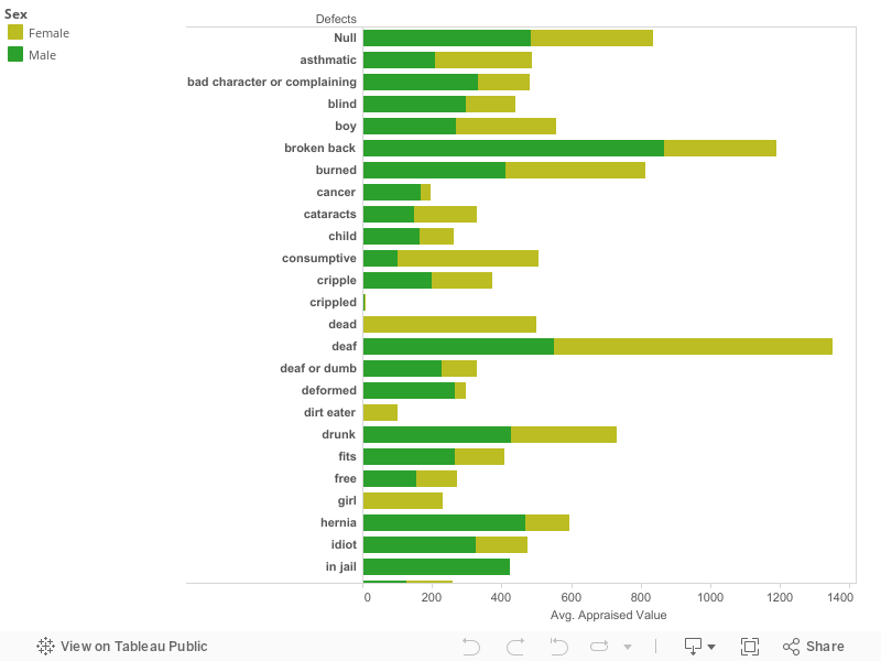
For the visualization I chose to compare the defects and sex of a slave and its affect on its appraisal value. I chose a bar graph to display the information because of its clarity and user friendliness. Looking at the graph we can see many factors that predetermine a slave’s value. For example, when comparing the sex of the slave, the appraisal value most of the time was lower for women then men. Also serious defects can affect a slave’s value more than others. On average a male slave in their prime was appraised at $734, pretty high compared to a male slave with cancer valued at $166. Most slaves were primarily sold to work and produce for growing plantations. Other times, when a master experienced a decrease in profits they would sell their best slaves to help with their economic struggles. It also did not help that as America began expanding the country, the opportunity to own land increased leading to the need for more slaves.
Based on the bar graph, there is a distinguished difference between male and female appraisal values and defects. The colors in the graph were very important to me as well, I used gender centered colors blue and pink to clearly represent male and females respectively, so viewers would see the changes in appraisal value. When comparing defects of slave’s men and women often had a broad range for what could account for a defect. For example, there were defects that include dirt eater, runaway, and idiot, all “defects” that can carry a different representation to others. Women showed most value when they were pregnant or very fertile, as slave masters like to impregnate females as a form of production. As far as comparing defects men and women share many of the same. Some of the things listed as defects are blatantly racist. With defects listed like dumb, run away, and drunk its clear this data set represents a time where blacks were seen as less than whites. The state a slave was sold in also seemed to affect what defect they had. This indicates that the geographic location had some type of effect on how slaves became defected. I also noticed children are priced significantly lower than a prime male slave, so much so being a child is listed as a defect. One problem I did have with this data set was the fact a male slave in his prime on average was valued at $100 lower than a male slave with a broken back. This issue makes me question some of the true values of slaves with defects. Another issue was the amount of defects listed; Some of the defects can easily be grouped together to fix some of the clutters. Others like dirt eater need more research to determine what exactly the defect is.
Argumentation 1
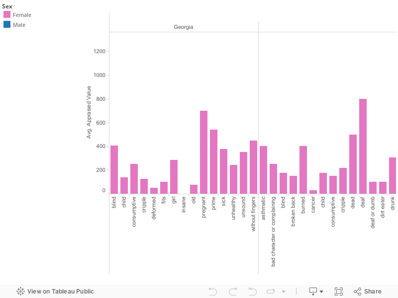
The visualization shows which types of defects different slaves had across the map of the several different states listed in the data set. The visualization is color coded by the different sexes that appear in the slave sales records for each of the listed states. You can make the case that since some states were more labor intensive then others, defects varied for slaves at different geographic locations.
When looking at the graph you can see differences in types of defects that appear to be more common compared to defects in other states. For example, we are able to see that in the more northern states, the slaves that were listed as having defects appeared to be defects such as being lame, blind, or having a bad attitude. This is compared to a southern state such as the booming cotton kingdom in Louisiana where not only does it contain all of the previously listed defects, but it also primarily contains physical defects that are most likely attributed to the intense labor and living conditions that they were forced to endure. Some defects included conditions such as being crippled, broken back, or a hernia, broken back. These labor conclusive defects/injuries seem to be more prominent in the further down south states then the further up states. This could be because over time, the labor the slaves endured wore them down and ultimately led to physical injuries that caused them to be listed as defected.
Also in this dataset a variety of defects do not become listed till the start of the 1800s. This could be because the types of labor that slaves were forced to endure were not as dehumanizing as further north states. Slaves with a less workload did not develop defects in the more northern slave states until later in the 19th century. It seems as time proceeded and the slavery industry began to expand more and more, slaves with defects began to appear more towards the north later in time because they were being sold with defects at a faster rate then ever. With the importance of a “prime” enslaved person in the south many slaves with defects were being auctioned to states further up north. This conclusion is supported in the dataset by looking at the defects that appear in the states mentioned above such as Mississippi. Most of the defects that do appear in further north states like Mississippi are not anything that would be too physically dependent. Some defects include being sick, “lame”, old, or run away. These are all debatable “defects” that could easily be fixed with proper care and time, but since slaves were not treated as humans but as property that can gain and lose value, small “defects” can determine what part of the country a slave lands in America.
Process Documentation
With a dataset like Slave Sales, interpretation is important so when going about visualization, the proper message had to be relayed. My use of a couple different kinds of graphs and maps for the dataset was meant not to be too uniform and pop to the viewer. The two visualizations that I have focused on are the bar graphs and tree maps. The first visualization type that I chose to use was the bar graph. I believe the bar graph is one of the simplest and best methods to display data visualization. It’s simple to understand and very user friendly. I use the bar graph to compare several categories involved in slave trade such as the state the slave was sold in, such as differences in sexes between the slaves in the data set, the appraisal value of the slaves, and defects a slave possessed.
Another visualization I used was the tree maps. Very different compared to the other graphs available, the tree map turned out to be very effective. With this graph I was able to compare the skills of each slaves and determine if the sex had any effect on the skillset. The tree map made it much easier to display this information to the viewer with a clear message. As the sex of the gender started to change the boxes in the tree maps skill sets progressively got smaller, concluding that female skills were generally valued less than males. In regards to the color chosen for the bar graphs, it was easiest and clearest to chose gender based colors blue and pink to compare defects and sex of different slaves. As far as the tree map data that displayed the skill sets and sex of the dataset, I chose the color red simply because that is what I associate slavery with; also red relays the message I would like viewers to visualize, the gruesome history behind slavery. The bar graph overall may be the best method for comparing the data that I have used for this dataset. The bar graph helps argue that slaves defects and sex effected what they were appraised for and in most case where they were purchased.
I also tried to create a symbol map to try to compare the relationship between states a slave was sold at and a defect carried. I noticed more and more states further north had defects that wouldn’t produce in plantations. For example, a blind slave can be of no value to a plantation owner but someone further up north, the slave can assist in other things. The symbol map with more information on slave sales of different states would also serve as a great way to visualize where different slaves with different defects were being sold to; as run away slaves and physically defected slaves by hard labor are more likely to be sold up north.
Argumentation 2
The Data set of the Slave Sales from 1775 to 1865 contain different columns that identify a slave and which one of seven southern states they were sold in. Looking at the graph there is a clear sequence in the data set. Comparing the gender, age, and value, it is possible to pin point how each of these categories effect appraisal value of a slave.
A male slave at his prime is usually around the age of 18-30 and on average pulls in almost $800 at auction, around $20,000 in todays cash. Age also plays a major factor in appraisal value, around the age of 40 the appraised value of a male drops sharply with the average appraised value being around $600. The decline in price can most likely be associated with growing health concerns and inability to produce hard labor as an enslaved person gets older and older. Essentially slaves old age become a liability rather than aid, it is evident in the fact a 99-year-old male slave was appraised at $19.
For comparison the average value for a “prime/fertile” female slave in the data set was around $567, almost $21,000 in todays cash. Unlike a male, a females peak ages are cut shorter. After the age of twenty-nine the value of a female slave drastically drops. The lowest average value for a female slave is an elderly just like a male. Children are also sold for cheap too but generally more than elderly. It is arguable through the dataset that women had gender specified roles that typically centered around child bearing and house chores. The labor roles of the enslaved men were a huge part in the South’s economics, making them more valuable then women.
Further Questions
Looking at this dataset we can get a glimpse of a horrible time that helped shaped America’s history. Reading the information in the dataset and seeing what constitutes as a defect for a slave brings the history to life for me. In every way whites tried to dehumanize African Americans even on record. I didn’t consider the fact that no names were attached to the skill sets and defects of the enslaved, rather treated as a form of property. The fact that being a child was listed as a defect indicate how the slave trade tore families apart.
Looking at all the different factors in the dataset, it became easier to see the correlate certain things with others. For example, the records show how slaves were being appraised and what might have influenced the increase or decrease in value. One thing I would like to understand better would be a better insight to the process slaves were sold. Where were the auctions held? How would one be able to evaluate a slave past someone’s word? Were the best slaves advertised or “praised”?
How slaves acquired some of their skills were astonishing to me. Given that slaves weren’t allowed to read and write they still were taught some very hard trades including blacksmith and mechanics. What predetermines what skill set will be taught to a specified slave?
With this dataset there are only so many questions answered about slavery. To find answers to some of my questions further research would be required. I would start by looking at more northern states for comparison to the seven southern states of this dataset. Based on geographic location looking at slave datasets for states like Maryland and Pennsylvania, we can view similarities and differences in things like skill sets. We can see where on the map most skills sets were increased and were on the map certain skills were nonexistent. Given that the north was more industrialized in the United States than the south, I was curios to if the skill sets of women would change in different datasets from the “domestic” centered skill sets of the south. I also wonder if the appraised value of these slaves was affected by industrialization just as much as the cotton boom affect value of a slave in southern states. Some ways to go about researching this information would be to look at a census and see how the slave sale categories compared to the more industrialized states up north. Personal slave accounts would probably reassure the question of How slaves felt working as a form of property. Letters from slaves either from the north or south can determine what hardships, if they faced and if they were dehumanized in any facet. Focusing on defects in the visualization, what affect does gender have on treatment of defects, if any? Is there any health coverage a master would put on his most productive slaves, which in most cases are men or is the value of every slave important to an owner? Based on the previous examples of sexism faced by slaves by looking at differences in appraised value between males and females, it would make more common sense to conclude that top notch male slaves receive more medical attention than a female with a defect. To prove this theory, further research on the medical attention that was given to slaves during this time period and attempt to specifically locate scholarly reviewed sources and recorded history about treatment of defects.